Database Join Algorithms: The Hidden Mechanics Behind SQL Query Execution

Exploring Nested Loop, Merge, and Hash Join Strategies Through Real-World Implementation Analysis

Every SQL query containing a JOIN clause triggers complex algorithmic decisions within the database engine. While developers focus on writing declarative SQL statements, the engine must choose from several fundamental strategies to combine data from multiple tables efficiently. This technical exploration examines how PostgreSQL, MySQL, and other relational databases implement the three core join algorithms. Also, as much as I know MySQL does not support Merge Join (also known as sort-merge join).

The Working Example: E-commerce Order Processing

Consider an e-commerce platform with two critical tables. The customers table stores user account information, while the orders table tracks purchase history. Each order connects to a customer through a customer_id foreign key relationship.

-- Query to analyze customer purchasing patterns
SELECT customers.email, customers.region, COUNT(orders.id) as order_count, 
       SUM(orders.total_amount) as total_spent
FROM customers 
INNER JOIN orders ON customers.id = orders.customer_id
WHERE orders.created_date >= '2024-01-01'
GROUP BY customers.email, customers.region
ORDER BY total_spent DESC;

This query demonstrates typical join scenarios encountered in production systems. The database engine must evaluate multiple algorithmic approaches to execute this operation efficiently.

Algorithm 1: Nested Loop Join Implementation

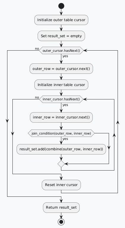
The nested loop join algorithm provides the most intuitive approach to combining tables. It systematically compares every row from the first table against every row from the second table.

Core Algorithm Structure

The implementation follows a straightforward nested iteration pattern:

1. Outer Relation Scan: Process each row from the driving table

2. Inner Relation Scan: For each outer row, examine all inner table rows

3. Predicate Evaluation: Test join conditions for each row combination

4. Result Assembly: Collect matching row pairs into the output set

Performance Analysis and Optimization

Computational Complexity: O(n × m) where n represents customers table size and m represents orders table size.

Memory Requirements: O(1) since no intermediate data structures are needed.

Optimization Opportunities:

• Index-based inner table access transforms full scans into targeted lookups

• Block-based processing reduces I/O operations

• Early termination when join conditions cannot be satisfied

Practical Implementation Details

-- Conceptual nested loop execution for customer orders
FOR each customer_row IN customers DO
    FOR each order_row IN orders DO
        IF customer_row.id = order_row.customer_id THEN
            IF order_row.created_date >= '2024-01-01' THEN
                OUTPUT (customer_row.email, customer_row.region, 
                       order_row.total_amount)
            END IF
        END IF
    END FOR
END FOR

Modern database systems enhance nested loop performance through sophisticated indexing strategies. When a B-tree index exists on orders.customer_id, the algorithm transforms from O(n × m) to O(n × log m), dramatically improving execution time.

Algorithm 2: Merge Join Strategy

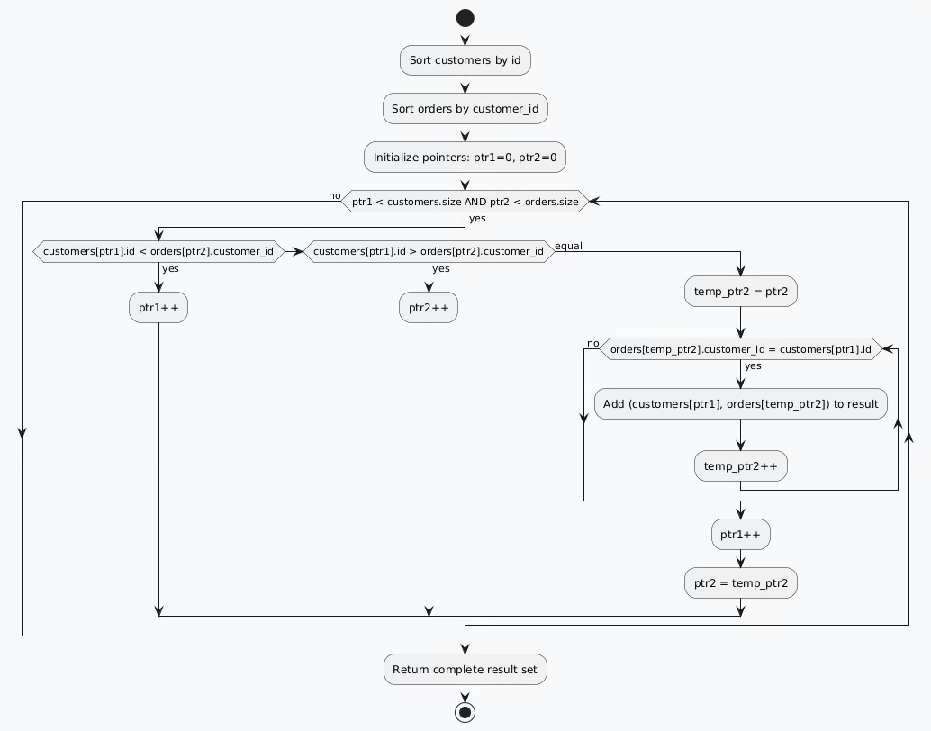
The merge join algorithm leverages the efficiency of merging sorted sequences, similar to the merge phase of merge sort. This approach excels when dealing with large datasets that can be efficiently sorted.

Algorithmic Execution Flow

Merge joins operate through distinct phases:

1. Sort Phase: Order both tables by their join attributes

2. Merge Phase: Simultaneously traverse sorted relations

3. Match Phase: Generate output for equivalent join keys

Performance Characteristics

Time Complexity: O(n log n + m log m) for sorting, followed by O(n + m) for merging.

Space Complexity: O(n + m) for storing sorted intermediate results.

Optimal Conditions:

• Large datasets where sorting costs are amortized across multiple operations

• Pre-existing sorted order through clustered indexes

• High join selectivity with evenly distributed keys

Advanced Implementation Considerations

-- Conceptual merge join execution
-- Assume sorted inputs: customers_sorted, orders_sorted
customer_ptr = 0
order_ptr = 0

WHILE customer_ptr < customers_sorted.length AND 
      order_ptr < orders_sorted.length DO
    
    current_customer = customers_sorted[customer_ptr]
    current_order = orders_sorted[order_ptr]
    
    IF current_customer.id < current_order.customer_id THEN
        customer_ptr++
    ELSIF current_customer.id > current_order.customer_id THEN
        order_ptr++
    ELSE
        -- Process all orders for this customer
        WHILE orders_sorted[order_ptr].customer_id = current_customer.id DO
            OUTPUT (current_customer, orders_sorted[order_ptr])
            order_ptr++
        END WHILE
        customer_ptr++
    END IF
END WHILE

The merge join algorithm particularly benefits from database systems that maintain sorted indexes. When a clustered index exists on the join column, the sorting phase becomes unnecessary, reducing complexity to O(n + m).

Algorithm 3: Hash Join Implementation

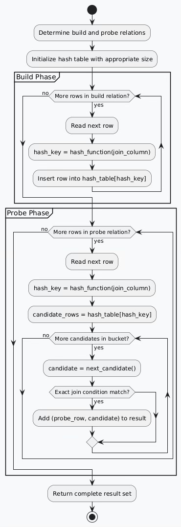
Hash joins represent the most sophisticated approach, utilizing hash tables to achieve optimal performance for equi-joins. This algorithm particularly excels with large datasets where one table is significantly smaller than the other.

Two-Phase Execution Model

Hash joins execute through carefully orchestrated phases:

1. Build Phase: Construct hash table from smaller relation

2. Probe Phase: Scan larger relation, performing hash lookups

Hash Function Design and Performance

Average Case Complexity: O(n + m) with uniform hash distribution.
Worst Case Complexity: O(n × m) when hash collisions create skewed buckets.
Memory Requirements: O(min(n, m)) for hash table storage.

Practical Hash Join Implementation

-- Conceptual hash join execution
-- Build phase: Create hash table from customers (smaller table)
hash_table = {}
FOR each customer_row IN customers DO
    hash_key = hash_function(customer_row.id)
    hash_table[hash_key].append(customer_row)
END FOR

-- Probe phase: Scan orders table
FOR each order_row IN orders DO
    hash_key = hash_function(order_row.customer_id)
    candidate_customers = hash_table[hash_key]
    
    FOR each candidate IN candidate_customers DO
        IF candidate.id = order_row.customer_id THEN
            OUTPUT (candidate, order_row)
        END IF
    END FOR
END FOR

Advanced Hash Join Variants

Modern database systems implement sophisticated hash join variations:

Grace Hash Join: Partitions data when hash tables exceed available memory, using disk-based processing for large datasets.

Hybrid Hash Join: Combines in-memory and disk-based approaches, keeping frequently accessed partitions in memory.

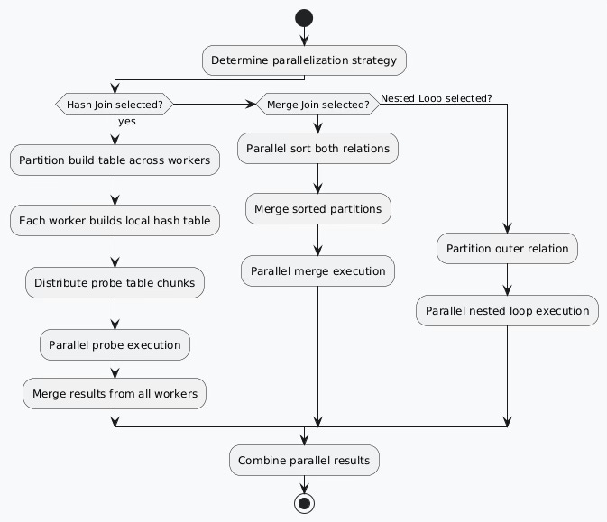
Parallel Hash Join: Distributes hash table construction and probing across multiple CPU cores.

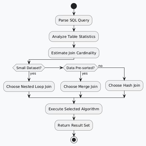
Query Optimizer Decision Framework

Database query optimizers employ cost-based models to select optimal join algorithms. The decision process considers multiple factors simultaneously.

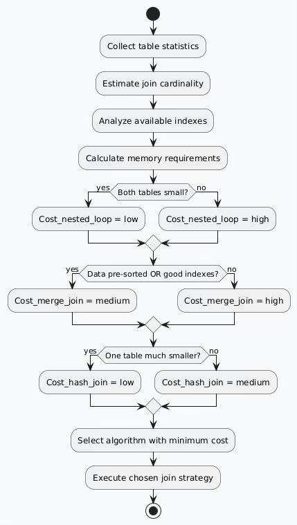
Cost Estimation Factors

Database systems maintain comprehensive statistics for accurate cost modeling:

Table Statistics: Row counts, average row sizes, data distribution patterns Index Properties: Selectivity ratios, clustering factors, index depth System Resources: Available memory, CPU capabilities, I/O bandwidth Query Characteristics: Selectivity predicates, result set size estimates

Performance Optimization Strategies

Index Design Principles

Each join algorithm benefits from specific indexing strategies:

Nested Loop Optimization: Create indexes on inner table join columns to eliminate full table scans.

Merge Join Enhancement: Utilize clustered indexes that maintain natural sort order on join attributes.

Hash Join Acceleration: Index build table join columns to reduce I/O during hash table construction.

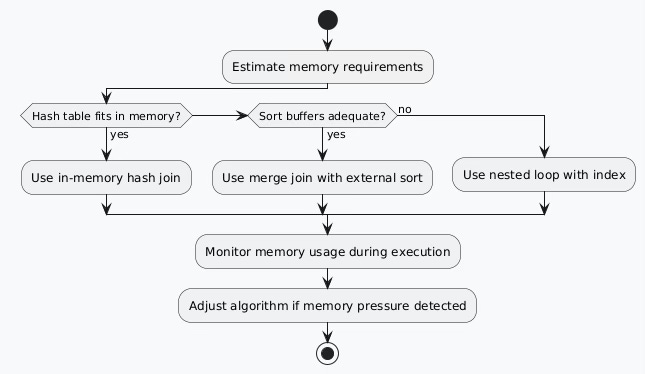
Memory Management Considerations

Real-World Performance Implications

Benchmark Scenarios

Consider performance characteristics across different data scales:

Small Datasets (< 10K rows): Nested loop joins often outperform more complex algorithms due to lower setup costs.

Medium Datasets (10K-1M rows): Algorithm choice depends heavily on index availability and data distribution.

Large Datasets (> 1M rows): Hash joins typically provide optimal performance for equi-joins, while merge joins excel with sorted data.

Query Writing Best Practices

-- Optimized query structure
SELECT c.email, c.region, 
       COUNT(o.id) as order_count,
       SUM(o.total_amount) as total_spent
FROM customers c
INNER JOIN orders o ON c.id = o.customer_id
WHERE o.created_date >= '2024-01-01'
  AND c.region IN ('North', 'South', 'East', 'West')
GROUP BY c.email, c.region
ORDER BY total_spent DESC;

Optimization Techniques:

• Place most selective predicates first in WHERE clauses

• Use appropriate data types for join columns

• Maintain current table statistics

• Consider covering indexes for frequently joined columns

Advanced Implementation Details

Parallel Processing Integration

Modern database systems incorporate parallel processing into join algorithms:

Adaptive Query Execution

Contemporary database systems implement adaptive optimization that adjusts join strategies during execution based on actual data characteristics encountered.

Conclusion

Database join algorithms represent sophisticated engineering solutions to fundamental data processing challenges. While nested loop joins provide simplicity and predictability, merge joins offer excellent performance for sorted data, and hash joins excel with large-scale equi-join operations.

Understanding these algorithms enables database developers to write more efficient queries, design better schemas, and make informed decisions about indexing strategies. The choice between these approaches can determine whether a query executes in milliseconds or minutes.

Modern database systems continue advancing these core algorithms through parallel processing, adaptive optimization, and intelligent memory management. However, the fundamental principles remain constant: organize data strategically, choose algorithms based on data characteristics, and leverage the query optimizer's sophisticated decision-making capabilities.

The next time you write a JOIN statement, consider the algorithmic complexity working behind the scenes to deliver your results efficiently. These time-tested algorithms form the foundation of every successful database-driven application.